
Calculating Pigouvian Taxes and Marginal Social Benefit (MSB) Equilibrium in IB Economics Paper 3
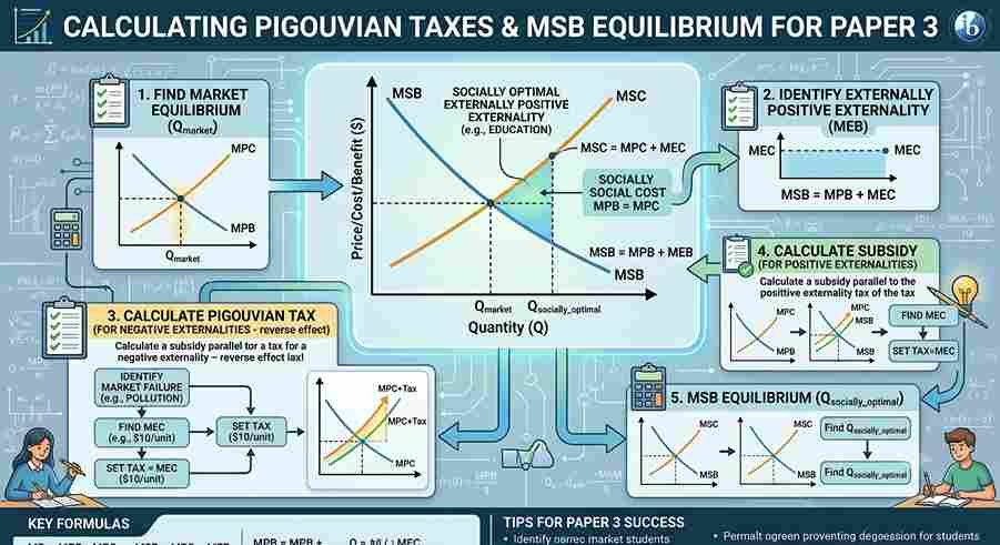
Last Updated: October 2026 | By EdFlik Team
For Higher Level (HL) students completing the International Baccalaureate (IB) Economics course, Paper 3 (Policy Paper) represents an intensive quantitative and analytical test. Among the core quantitative topics tested, calculating market failure equilibria, negative production externalities, and optimal Pigouvian taxes based on Marginal Social Benefit (MSB) and Marginal Social Cost (MSC) functions routinely appears across section A and B items.
Students frequently drop marks on Paper 3 not due to conceptual misunderstandings of externalities, but because of algebraic errors: confusing private and social curves, miscalculating deadweight loss triangles, or failing to evaluate the precise vertical distance required for a carbon/excise tax.
This comprehensive, exam-focused masterclass guide breaks down the underlying welfare mathematics, provides a step-by-step calculation workflow, walks through a fully worked numerical model, exposes top examiner traps, and supplies a 100% copy-paste JSON-LD schema markup for your study resources.
Part 1: Mathematical Foundations of Externalities
In a free market experiencing negative production externalities (such as industrial pollution or carbon emissions), private agents fail to account for the costs imposed on third parties. To evaluate market equilibrium and design optimal policy corrections, we define four core curves algebraically:
                  CORE ALGEBRAIC CURVES IN EXTERNALITIES
                                     |
        +----------------------------+----------------------------+
        |                                                         |
1. MPB (Marginal Private Benefit)                        2. MPC (Marginal Private Cost)
• Represents consumer demand: $P = f(Q)$.                 • Represents private supply: $P = f(Q)$.
• Assumes no consumption externalities ($\text{MPB} = \text{MSB}$). • Direct costs borne directly by producers.
        |                                                         |
        +----------------------------+----------------------------+
                                     |
        +----------------------------+----------------------------+
        |                                                         |
3. MSC (Marginal Social Cost)                            4. MEC (Marginal External Cost)
• $\text{MSC} = \text{MPC} + \text{MEC}$.                  • The external damage per unit imposed on society
• Total cost to society of producing one more unit.        (can be a flat constant or a function of output $Q$).
The Efficiency Condition:
- Free-Market Equilibrium: Occurs where private buyers meet private suppliers:$\text{MPB} = \text{MPC}$. This generates the free-market quantity ($Q_m$).
- Socially Optimal Equilibrium: Occurs where society's total benefits equal total costs:$\text{MSB} = \text{MSC}$. This generates the socially efficient quantity ($Q^*$), where $Q^* < Q_m$ for negative externalities.
Part 2: Step-by-Step Paper 3 Calculation Protocol
When faced with a quantitative externality and taxation question on Paper 3, execute this 6-step problem-solving sequence:
                  THE 6-STEP QUANTITATIVE CALCULATION PROTOCOL
                                   |
  Step 1: Find Free-Market Quantity ($Q_m$) ---> Set $\text{MPB} = \text{MPC}$ and solve for $Q$.
  Step 2: Derive MSC Function               ---> Add Marginal External Cost ($\text{MEC}$) to $\text{MPC}$.
  Step 3: Find Socially Optimal $Q^*$       ---> Set $\text{MSB} = \text{MSC}$ and solve for $Q^*$.
  Step 4: Calculate Optimal Pigouvian Tax   ---> Evaluate vertical gap ($\text{MSC} - \text{MPC}$) at quantity $Q^*$.
  Step 5: Determine Tax Revenue             ---> Multiply Tax Rate by the new post-tax quantity traded.
  Step 6: Compute Deadweight Loss (DWL)     ---> Calculate area of the welfare loss triangle $\left(\frac{1}{2} \times \text{base} \times \text{height}\right)$.
Part 3: Fully Worked Numerical Model
Exam-Style Problem:
Consider a chemical manufacturing market characterized by the following linear functions:Demand / Marginal Private Benefit ($\text{MPB} = \text{MSB}$): $P = 120 - 2Q$Supply / Marginal Private Cost ($\text{MPC}$): $P = 20 + 2Q$Marginal External Cost ($\text{MEC}$): Each unit produced imposes a constant external pollution damage of $\$20$ on local residents ($\text{MEC} = 20$).
Tasks:Calculate the free-market equilibrium price and quantity ($P_m, Q_m$).Derive the Marginal Social Cost ($\text{MSC}$) equation and calculate the socially optimal quantity ($Q^*$).Calculate the precise per-unit Pigouvian tax required to achieve social efficiency.Calculate total government tax revenue and the deadweight loss removed by the tax.
Step 1: Free-Market Equilibrium ($Q_m$)
Set$\text{MPB} = \text{MPC}$:
$$120 - 2Q = 20 + 2Q$$$$120 - 20 = 2Q + 2Q$$$$100 = 4Q \implies \mathbf{Q_m = 25 \text{ units}}$$
Substitute $Q_m = 25$ back into the demand equation to find market price ($P_m$):
$$P_m = 120 - 2(25) = 120 - 50 = \mathbf{\$70}$$
Step 2: Derive MSC and Find Socially Optimal Quantity ($Q^*$)
Add$\text{MEC}$ to$\text{MPC}$ to find$\text{MSC}$:
$$\text{MSC} = \text{MPC} + \text{MEC} = (20 + 2Q) + 20 = \mathbf{40 + 2Q}$$
Set$\text{MSB} = \text{MSC}$ to find the socially optimal allocation ($Q^*$):
$$120 - 2Q = 40 + 2Q$$$$120 - 40 = 2Q + 2Q$$$$80 = 4Q \implies \mathbf{Q^* = 20 \text{ units}}$$
Step 3: Calculate the Optimal Pigouvian Tax
A Pigouvian tax levied on producers shifts the private supply curve ($\text{MPC}$) vertically upwards by the exact amount of the external marginal damage evaluated at the socially optimal output:
$$\text{Tax per unit} = \text{MEC} = \mathbf{\$20 \text{ per unit}}$$
When a $\$20$ per-unit tax is imposed, the new private supply curve becomes:
$$\text{MPC}_{\text{tax}} = (20 + 2Q) + 20 = 40 + 2Q$$
Notice that$\text{MPC}_{\text{tax}}$ is now identical to$\text{MSC}$. Setting$\text{MPC}_{\text{tax}} = \text{MPB}$ internalizes the externality, forcing the market to settle precisely at$Q^* = 20$.
Step 4: Tax Revenue and Deadweight Loss Removed
- New Post-Tax Price Paid by Consumers ($P_c$): Substitute $Q^* = 20$ into the demand equation:$$P_c = 120 - 2(20) = \mathbf{\$80}$$
- Government Tax Revenue: Calculated as $\text{Tax Rate} \times Q^*$:$$\text{Revenue} = \$20 \times 20 \text{ units} = \mathbf{\$400}$$
- Deadweight Loss (DWL) Triangle Removed: The welfare loss triangle exists between the free-market quantity ($Q_m = 25$) and the social optimum ($Q^* = 20$):
- Base: $Q_m - Q^* = 25 - 20 = 5 \text{ units}$
- Height: Vertical gap between $\text{MSC}$ and $\text{MSB}$ at $Q_m = 25$
- $\text{MSC}(25) = 40 + 2(25) = 90$
- $\text{MSB}(25) = 120 - 2(25) = 70$
- $\text{Height} = 90 - 70 = \$20$
- DWL Area: $\frac{1}{2} \times \text{base} \times \text{height} = \frac{1}{2} \times 5 \times 20 = \mathbf{\$50}$
The Pigouvian tax successfully eliminates this $\$50$ deadweight loss, restoring allocative efficiency to the market.
Part 4: Top 4 Calculation Traps That Cost Students Marks in Paper 3
- Adding MEC to Demand Instead of Supply: Mistakenly shifting the demand curve ($\text{MPB}$) upward when dealing with a production externality. Negative production externalities affect costs, shifting$\text{MPC}$ upward to form$\text{MSC}$. Demand remains untouched unless it is a consumption externality.
- Evaluating the Tax at the Wrong Quantity: Calculating the Pigouvian tax using the free-market quantity ($Q_m$) rather than the socially optimal quantity ($Q^*$). When$\text{MEC}$ varies with output (e.g.,$\text{MEC} = Q$), the tax must be evaluated strictly at$Q^*$.
- Confusing Consumer Price with Producer Net Price: Failing to distinguish between the higher price consumers pay post-tax ($P_c$) and the net revenue producers receive after subtracting the tax ($P_p = P_c - \text{tax}$).
- Arithmetic Sign Errors in Simultaneous Equations: Dropping negative coefficients when rearranging linear equations, leading to impossible negative quantities or prices. Always double-check your simultaneous steps.
Frequently Asked Questions (FAQs)
Q1: How do I know whether to add or subtract MEC when deriving MSC?
Ans: For negative externalities, social costs are higher than private costs, so you always add Marginal External Cost ($\text{MEC}$) to Marginal Private Cost ($\text{MPC}$) to obtain$\text{MSC}$ ($\text{MSC} = \text{MPC} + \text{MEC}$).
Q2: Does a Pigouvian tax shift the demand curve or supply curve?
Ans: A indirect Pigouvian tax levied on producers shifts the supply curve ($\text{MPC}$) vertically upwards by the amount of the tax. It does not shift the demand curve.
Q3: What happens to deadweight loss when a Pigouvian tax is correctly implemented?
Ans: A correctly sized Pigouvian tax eliminates the deadweight loss entirely by forcing the market output to contract from$Q_m$ back to the socially efficient level$Q^*$, where$\text{MSB} = \text{MSC}$.