
Understanding Price Elasticity of Demand (PED) and Supply (PES) for IGCSE Economics
Last Updated: October 2026 | By EdFlik Education Team
For high school students completing the Cambridge IGCSE Economics (0455) or Edexcel IGCSE Economics (4EC1) qualifications, microeconomics forms the foundational pillar of the syllabus. Among all topics tested across Paper 1 (Multiple Choice) and Paper 2 (Structured Questions), few carry as much weight or appear as consistently as Price Elasticity of Demand (PED) and Price Elasticity of Supply (PES).
Whether analyzing how price changes impact business revenue, evaluating government intervention via indirect taxes and subsidies, or interpreting supply responsiveness during global supply chain disruptions, elasticities provide the mathematical and visual framework needed to explain market dynamics.
Every exam season, candidates lose marks not because they don't know the basic definitions, but because of common calculation errors: forgetting to divide percentage change in quantity by percentage change in price, dropping negative signs carelessly, or confusing elastic and inelastic curves on demand and supply diagrams.
In this comprehensive masterclass guide, our expert IGCSE economics educators break down the formulas, diagrammatic curves, determinants, business applications, and common exam traps to help you secure an $A^*$ grade.
Part 1: Price Elasticity of Demand (PED)
1. What is PED?
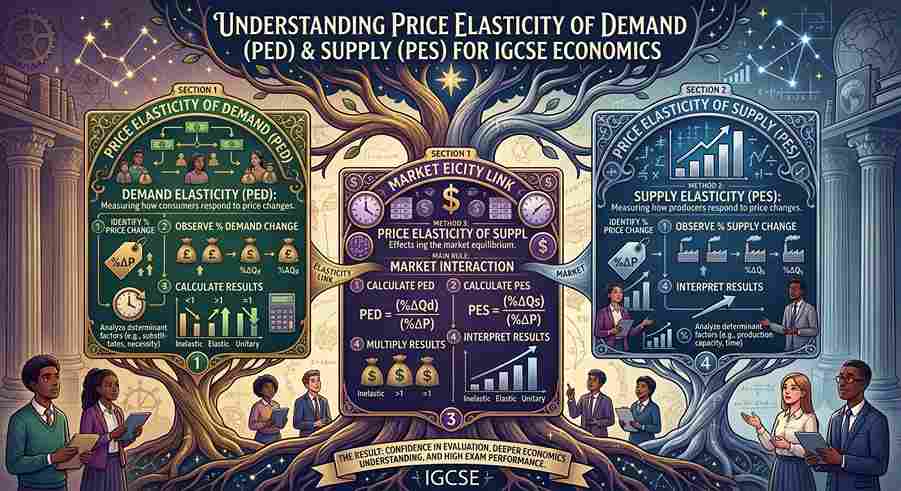
Price Elasticity of Demand (PED) measures the responsiveness of quantity demanded of a good or service to a change in its price.
The Fundamental Formula:
$$\text{PED} = \frac{\% \Delta \text{ Quantity Demanded}}{\% \Delta \text{ Price}}$$
Where:
$$\% \Delta = \left( \frac{\text{New Value} - \text{Original Value}}{\text{Original Value}} \right) \times 100$$
- The Sign Convention: Because demand curves obey the Law of Demand (as price increases, quantity demanded decreases), the resulting numerical value for PED is mathematically negative. In IGCSE Economics, we usually consider the absolute value (ignoring the minus sign) when evaluating elasticity.
2. Categories of Price Elasticity of Demand
                         PED ELASTICITY VALUES
                                   |
      +----------------------------+----------------------------+
      |                            |                            |
  PED > 1                      PED < 1                      PED = 1
Price Elastic                Price Inelastic             Unitary Elastic
Sensitive to Price           Insensitive to Price       % Change in Qd = % Change in P
Shallow Demand Curve         Steep Demand Curve         Rectangular Hyperbola
- Price Elastic Demand ($\text{PED} > 1$): Quantity demanded changes by a proportionately larger percentage than the percentage change in price.
- Example: A $10\%$ increase in price causes a $20\%$ drop in quantity demanded ($\text{PED} = -2$).
- Price Inelastic Demand ($\text{PED} < 1$): Quantity demanded changes by a proportionately smaller percentage than the percentage change in price.
- Example: A $10\%$ increase in price causes only a $3\%$ drop in quantity demanded ($\text{PED} = -0.3$).
- Unitary Elastic Demand ($\text{PED} = 1$): Quantity demanded changes by the exact same percentage as the price change. Total revenue remains constant at all prices.
- Perfectly Inelastic Demand ($\text{PED} = 0$): Quantity demanded does not change at all regardless of price changes (vertical demand curve).
- Perfectly Elastic Demand ($\text{PED} = \infty$): Consumers will buy any quantity at a specific price, but quantity drops to zero if the price rises even slightly (horizontal demand curve).
3. Key Determinants of Price Elasticity of Demand (SPLATT Framework)
Why are some goods elastic while others are inelastic? Memorize the SPLATT acronym for IGCSE structured questions:
- S — Substitutes: Availability and closeness of substitutes. If many close substitutes exist (e.g., brand A vs. brand B coffee), demand is elastic. If no close substitutes exist (e.g., life-saving insulin or water), demand is inelastic.
- P — Proportion of Income: Goods that take up a large proportion of a consumer's household budget (e.g., cars, holidays) have elastic demand. Goods taking up a negligible proportion (e.g., salt, matches) have inelastic demand.
- L — Luxury vs. Necessity: Luxuries (e.g., designer watches, sports cars) are non-essential, making demand elastic. Necessities (e.g., basic staple foods, electricity) are essential, making demand inelastic.
- A — Addictiveness / Habit-forming: Goods that are habit-forming or addictive (e.g., cigarettes, alcohol, caffeine) have highly inelastic demand because consumers find it difficult to reduce consumption even when prices rise.
- T — Time Period: In the short run, demand is often inelastic because consumers need time to adjust their habits or find alternatives. In the long run, demand becomes more elastic as consumers adapt and switch to substitutes.
4. PED and Total Revenue (Essential for Business Applications)
Understanding PED allows businesses to make strategic pricing decisions to maximize Total Revenue ($\text{TR} = \text{Price} \times \text{Quantity}$):
| Elasticity Type | Price Action | Effect on Quantity Demanded | Effect on Total Revenue (TR) |
| Elastic ($\text{PED} > 1$) | Lower Price | Quantity increases by a larger $\%$ | TR Increases |
| Elastic ($\text{PED} > 1$) | Raise Price | Quantity decreases by a larger $\%$ | TR Decreases |
| Inelastic ($\text{PED} < 1$) | Raise Price | Quantity decreases by a smaller $\%$ | TR Increases |
| Inelastic ($\text{PED} < 1$) | Lower Price | Quantity increases by a smaller $\%$ | TR Decreases |
IGCSE Exam Tip: If a product has inelastic demand (e.g., electricity or tobacco), the firm should increase the price to raise total revenue because the price increase outweighs the small drop in sales volume!
Part 2: Price Elasticity of Supply (PES)
1. What is PES?
Price Elasticity of Supply (PES) measures the responsiveness of quantity supplied of a good or service to a change in its price.
The Fundamental Formula:
$$\text{PES} = \frac{\% \Delta \text{ Quantity Supplied}}{\% \Delta \text{ Price}}$$
- Positive Value: Because supply curves follow the Law of Supply (as price increases, producers are incentivized to supply more), PES is almost always positive.
2. Categories of Price Elasticity of Supply
- Price Elastic Supply ($\text{PES} > 1$): Quantity supplied changes by a proportionately larger percentage than the price change (flatter supply curve passing through the vertical price axis).
- Price Inelastic Supply ($\text{PES} < 1$): Quantity supplied changes by a proportionately smaller percentage than the price change (steeper supply curve passing through the horizontal quantity axis).
- Unitary Elastic Supply ($\text{PES} = 1$): Any straight-line supply curve that passes directly through the origin $(0,0)$ has a PES of 1.
- Perfectly Inelastic Supply ($\text{PES} = 0$): Quantity supplied cannot be changed regardless of price changes (vertical supply curve, e.g., seats in a sports stadium or fresh agricultural harvest on market day).
3. Key Determinants of Price Elasticity of Supply (TASTE Framework)
How quickly can producers increase output when market prices rise? Use the TASTE framework:
- T — Time Period: In the immediate market period, supply is perfectly inelastic because producers cannot adjust production instantaneously. In the short run, supply becomes more responsive as variable inputs (labor, raw materials) are adjusted. In the long run, supply is highly elastic as firms expand factory capacity or enter the market.
- A — Availability of Spare Capacity: If a factory operates with unused machinery or excess capacity, it can rapidly increase output when prices rise ($\text{PES} > 1$). If operating at $100\%$ capacity, supply is inelastic ($\text{PES} < 1$).
- S — Stocks of Finished Goods / Inventory: If a business holds large inventories of finished goods or raw materials, it can release them onto the market immediately when prices rise ($\text{PES} > 1$). Perishable items (e.g., fresh fruit, milk) cannot be stored easily, making supply inelastic.
- T — Time to Produce / Production Lag: Goods that take a long time to manufacture or cultivate (e.g., agricultural crops requiring seasonal growth, mining crude oil) have inelastic supply. Goods with rapid production cycles (e.g., mass-produced plastic toys, digital services) have elastic supply.
- E — Mobility of Factors of Production: If workers, capital, and raw materials can easily be switched from producing one good to another (e.g., a bakery switching from baking bread to cakes), supply is elastic.
Part 3: Top 4 Traps That Cost Students Marks in IGCSE Economics
- Flipping the Elasticity Formulas: Writing $\frac{\% \Delta \text{ Price}}{\% \Delta \text{ Quantity}}$ instead of $\frac{\% \Delta \text{ Quantity}}{\% \Delta \text{ Price}}$. Always remember: Quantity is on TOP!
- Confusing Inelastic with Perfectly Inelastic: Describing inelastic demand ($\text{PED} < 1$) as a situation where quantity demanded never changes. Quantity does change, just by a smaller percentage than price. Only perfectly inelastic ($\text{PED} = 0$) means quantity remains completely unchanged.
- Forgetting to Connect PED to Indirect Tax Burden: On Paper 2, when analyzing indirect taxes (e.g., sales tax or VAT), failing to state that when demand is inelastic, the tax burden falls mainly on the consumer, whereas when demand is elastic, the burden falls mainly on the producer.
- Mishandling Percentage Change Calculations: Calculating simple change (e.g., $\$5 - \$4 = \$1$) instead of percentage change ($\frac{\$1}{\$4} \times 100 = 25\%$). Always calculate percentage changes before applying elasticity formulas!
Preparing for Cambridge or Edexcel IGCSE Economics exams and aiming for an $A^$ grade? EdFlik connects international school students globally with expert, 1-to-1 online IGCSE tutors, helping you master microeconomic theory, data response questions, structured essay formats, and past-paper mark scheme techniques. *Book a Free Demo Class Today!
Frequently Asked Questions (FAQs)
Q1: Is PED constant along a straight-line demand curve?
Ans: No! This is a classic advanced question. Along a downward-sloping, straight-line demand curve, PED varies continuously. At higher prices (near the top left), demand is price elastic ($\text{PED} > 1$). At the midpoint, demand is unitary elastic ($\text{PED} = 1$). At lower prices (near the bottom right), demand becomes price inelastic ($\text{PED} < 1$).
Q2: Why do governments tax goods with inelastic demand like petrol, alcohol, and cigarettes?
Ans: Governments impose high indirect taxes on goods with inelastic demand for two main reasons:
- High Tax Revenue: Because consumers continue buying the product despite higher prices, the government generates substantial and reliable tax revenue.
- Market Failure Correction: Products like cigarettes and petrol generate negative externalities (pollution, health risks). Taxes raise prices to internalize these social costs.
Q3: What is the difference between PED and Cross Price Elasticity of Demand (XED)?
Ans: PED measures how quantity demanded of a product responds to changes in its own price. XED measures how quantity demanded of one product (Good A) responds to a change in the price of a related product (Good B), identifying whether goods are substitutes ($\text{XED} > 0$) or complements ($\text{XED} < 0$).
Q4: How does EdFlik support IGCSE Economics students?
Ans: EdFlik connects international school students worldwide with vetted, expert 1-to-1 online tutors specializing in Cambridge (0455) and Edexcel (4EC1) IGCSE Economics. Our personalized coaching focuses on clarifying market mechanisms, practicing calculation problems, structuring 6-mark and 8-mark data response questions, and working through past papers.